You are in: Instruments > Altair > Performance and Use > Commissioning Performance

Altair Commissioning Performance

Note: below are some initial performance plots. More data will be added as they become available.

Numerous images have been acquired during the past commissioning run. The following plots are derived from these data. Performance will evolve as some problems are fixed (in particular the vibration problem), but these results show a snapshot of Altair's current capabilities.

AO Crash Course

The performance of an adaptive optics system is fully defined by the output PSF at a given point in time. However, the performance can be approximated by a few parameters:

Strehl Ratio (the ratio of the maximum of the PSF over the maximum of the fully diffraction limited image, both images being normalized to the same total flux)
The Full Width at Half Maximum (FWHM)
The encircled energy

These parameters vary with:

The seeing, or r0. Note that the following relation apply:

FWHM [in arcsec] = lambda / [r0*4.848e-6]
r0(lambda) = r0(500nm)*(500/lambda[nm])^1.2

The coherence time of the atmosphere, tau0. This is usually difficult to determine, and is not a parameter determined in real time by Altair
The brightness of the guide star, mGS. Limited number of photons induce noise in the wave-front sensing, and part of this noise is injected in the output compensated wavefront
The distance to the GS, theta. This is usually called anisoplanatism
Several system parameters, including the number of actuators, sampling time, loop control scheme and gains, etc...

Each of these contributions (r0, tau0, isoplanatism, noise) contribute to compensated image quality. Their effect on the Strehl ratio is approximately cumulative (for Strehl ratio value > 0.1), i.e.
Strehl_total = constant * Strehl_r0 * Strehl_tau0 * Strehl_noise * Strehl_anisoplanatism

For more detailed information, please read the Adaptive optics pages.

The following plots are indicative of the current Altair performance and are given for information purposes. It is not expected that they be used by astronomers applying for time to predict exposure time, etc... For this task, please use the Integration Time Calculator.

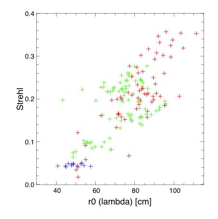
Figure 1: Strehl ratio versus r0 (JHK)
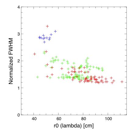
Figure 2: "Normalized" FWHM versus r0 (at JHK)
Figure 3: FWHM versus r0 (at K only)
Figure 4: 50% encircled energy radius versus r0 (at K)
Figure 5: Strehl versus distance to guide star (H band)

Figure 1: Strehl ratio versus r0 at the imaging wavelength. Data extracted from J (blue), H (green) and Kshort or Kprime (red) images. Note that r0 varies as lambda^1.2.

Figure 2: "Normalized" FWHM versus r0 at the imaging wavelength. The normalized FWHM is defined as the FWHM divided by the FWHM of a purely diffraction limited image (= lambda/D). Data extracted from J (blue), H (green) and Kshort or Kprime (red) images. Note that r0 varies as lambda^1.2.

Figure 3: Similar to figure 2; The K band images FWHM is plotted against r0(K).

Figure 4 (above): 50% encircled energy radius versus r0 at the imaging wavelength. Data extracted from Kshort or Kprime images. Note that r0 varies as lambda^1.2. Encircled energy is indicative but not directly relevant to all problems. For instance, for photometry of stellar objects in a cluster, a more relevant metric is the energy in the core (i.e. roughly lambda/D). The latter is approximately equal to the Strehl ratio, scaled by a geometric factor (percentage of energy in the core for a perfectly diffraction limited image) which is equal to 0.8. For instance, for a typical correction at H band, we have S=0.2 and therefore we have in the image core 0.2*0.8=0.16 of the total flux.

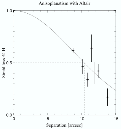Figure 5 (above): Effect of anisoplanatism with Altair. This plot displays the Strehl loss due to off-axis anisoplanatism only, expressed at H band, as a function of the distance to the guide star. Each data point is for a series of images (sequence) on a given double star. For each double star, we have a set of values; the data point is the average of these values, the error bar is the rms of these values. The smooth line is a simple fit: y=exp(-(x/12.5)^2). 50% Strehl attenuation occurs at a separation of 10.5 arcsec. As one can express the Strehl as the exponential of the phase variance and the phase variance obviously varies as lambda^2, the separation for which one gets 50% Strehl loss scales as the wavelength, i.e. one gets 8" at J and 14" at K.

Last update July 2, 2003; Jean-Pierre Véran and Francois Rigaut