GNIRS in the Observing Tool

It is recommended that you build your GNIRS observations using the OT library templates which provide sequences for all of the GNIRS instrument observing modes. Below is a guide to using the OT library, followed by detailed instructions on configuring GNIRS in the OT.

Instructions for using the OT library:

1) DECIDE on which GNIRS mode you need for your science. Consult the web pages for more information about the instrument capabilities that are offered.

2) CHOOSE whether you have a faint or bright science target. K = 14 is the boundary between the two cases.

3) SELECT the appropriate observation sequence (one of the blue groups) and paste this into your own phase II program. This is now your skeleton observation for a given science target at a given instrument configuration.

4) READ through all the notes in the group for more details about why the observations are set up as they are. Notice that in a scheduling group, the order of the observations defines the order in which they will be executed at the telescope.

5) UPDATE the target and GNIRS components (exposure time, coadds, position angle...) of all the science target and standard star observations within the group as necessary for your program and remove any unnecessary calibrations (e.g. J and H band cals for a K-band observation).

6) TELLURICS and other nighttime calibration observations are included within the group. End of night calibrations can be found within organizational folders (yellow) at the end of the GNIRS OT library. They should be kept separate from the nighttime science and calibration observations.

There are 2 recommended methods to organize your observations:

A) Group tellurics (2 sets per observation-- before/after) and calibrations with the science observation and corresponding acquisition observations. Rename the group to the name of the science target. This approach is best when there are multiple configurations, and/or few science targets. (see OT library example)

B) Define tellurics and calibrations separately, to be reused for all targets. This approach is better when there are numerous targets using the same calibrations or same set of tellurics. Baseline cals (including tellurics) DO NOT need to be repeated for every science target, however they must be at least 1 for each instrument configuration. IT MUST BE CLEAR WHICH CALIBRATIONS (tellurics and flats/arcs) GO WITH WHICH OBSERVATIONS.

Baseline telluric observations should be given Class ="Nighttime Partner Calibration" (at the "Observe" level); additional tellurics or other non-baseline nighttime observations should be given Class="Nighttime Program Calibration" (i.e., charged to program). All science observations (but not the acquisitions) have Class="Science".

Phase II primary Components:

• GNIRS Component - to define 'static' configurations, including 
• Long-Slit, Cross-dispersed, IFU
• GNIRS Iterator - to construct and sequence different instrument configurations
• Offset Iterator - to construct dithering sequences

There is also specific information on:

• Acquisition Observations 
• Calibration Observations - flats and arcs

Note that the GNIRS OIWFS is not yet available for use.  However, the inner perimeter of the OIWFS FOV in the Position editor is often useful to see the acquisition imaging field of view. 

For example templates of typical GNIRS Observations (i.e. science and telluric observations, all acquisitions, and GCAL calibrations), go to the instrument OT library.  

More information and guidelines are available on the Observing Strategies page.  Highlights include:

• Anticipating instrument overheads 
• Planning your exposure times and total observation times
• Defining appropriate guide stars
  

Refer to the GNIRS instrument pages for general information about the instrument.  When you're done, don't forget to check the Checklist.  If you still have questions, submit a HelpDesk query.

GNIRS Static Component

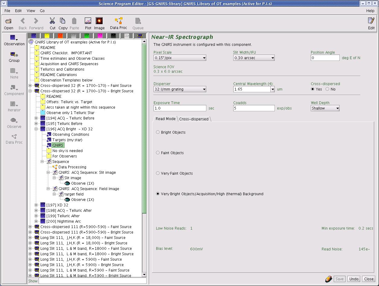
The detailed component editor for GNIRS is accessed by adding a GNIRS component to an observation, or adding a "GNIRS Observation".  The default screen looks like this:

The Wollaston prism is not yet available.  All other items must be set (see below for more details).  Briefly, these are:

• Pixel scale: determines which of the 2 types of cameras are used; 0.15"/pix is the short camera; 0.05"/pix is the long camera
• Exposure time & Coadds: minimum exposure time is 0.2sec, maximum exposure is generally dictated by object brightness or sky background (see Observing Strategies); coadds can be use to combine multiple integrations, especially useful in high background cases
• Disperser: chooses 1 of the 3 gratings available; this determines the resolution (in combination with pixel scale and slit width)
• Slit Width/IFU: the IFU is in the same mechanism as the slit widths.  The slit length is determined by a separate mechanism (the decker) which is implicitly determined based on other configuration information (pixel scale and cross-dispersion)
• Central Wavelength: sets the grating to achieve a particular wavelength near the center of your spectrum.  Menu choices are available (and strongly recommended) for moderate dispersion (0.15"/pix + 32 l/mm grating) configurations.  For higher dispersion, any wavelength can be entered.
• Cross-dispersed: Yes or No (not available with IFU or 0.05"/pixel scale).
• Position Angle: default is 0; other values, in degrees East of North can be entered.
• Well Depth: the bias voltage may be adjusted to modestly increase the well depth for thermal IR (L and M band) observations. Default is "shallow", appropriate for non-thermal IR (below 2.5 micron) observations.
  

Selecting cross-dispersed (XD) mode:

When the "Cross-dispersed" buttons are set to "Yes", the cross-dispersed tab becomes active (shown below).  This tab displays the full wavelength coverage provided by orders 3 through 8, the primary orders passed by the cross-dispersing prism.  (This is an informational tab only, no input is required.)  With pixel scale = 0.15 arcsec/pix and the 32 l/mm disperser (max. R~1700), the central wavelength should be set to "cross-dispersed" (=1.65um) and the observed spectrum provides essentially complete coverage from 0.9 to 2.5 um.

Pixel scale, disperser, slit width (including IFU and R=18000)

Choice of camera (pixel scale), dispersing element and focal plane mask (slit) is made by clicking on the pull down lists (i.e. the down-pointing arrows) and selecting the desired item. There are 2 pixel scales in GNIRS; 0.15"/pixel is provided by the "short" cameras while 0.05"/pixel is provided by the "long" cameras.  With the 0.15" pixel scale, the 32 l/mm grating (disperser) gives 2-pixel resolution of R~1700 (with the 0.3" slit) with complete coverage of the J, H, or K bandpasses in  single spectrum, while the 111 l/mm grating gives higher resolution (R~6000 in 2 pixels) with proportionally less wavelength coverage.  The 0.05" pixel scale increases these resolutions by a factor of 3 (with a 0.1" slit), along with 3x the spatial resolution (and the accompanying slit losses).  The 10 l/mm grating reduces the resolution a factor of 3 from the 32 l/mm grating and is not normally used.  A number of slit widths are available; slits wider than 2 pixels (0.3arcsec or 0.1arcsec with the long cameras) will reduce the effective resolution.  The slit length is determined separately and is fixed by the mode (99" for long slit with 0.15"/pix; 49" for long slit with 0.05"/pix; 6.1" for XD).  The science field of view (shown in green) will update to reflect the configuration chosen, also displayed by the position editor.

To define an IFU observation, set slit width = IFU.  The IFU can only be used with the 0.15/pix scale, and not in cross-dispersed mode of course.  Other items can be configured as desired.  Because the IFU provides a 2-dimensional FOV, the offset sequences can offset in p and q.  See the IFU page for more information.

To use the highest (spatial or spectral) resolution, select the 0.05"/pix pixel scale.  For R~18000, this pixel scale must be combined with the 111 l/mm grating.

Selecting a wavelength

The central wavelengths for each band when using the 32 l/mm disperser with the 0.15 arcsec pixel scale (R~1700; including cross-dispersed) are provided as a menu in the "central wavelength" window; it is strongly recommended that the menu wavelengths be used for this configuration.  For R~6000 and 18000, one can also enter a specific wavelength in this window.  The number in parentheses to the right of "Central Wavelength" indicates the order associated with that wavelength. Note that the proper order-sorting filter is automatically selected based on the central wavelength.  When "Cross-dispersed" is set to "Yes", the Cross-dispersed tab will show the wavelength coverage provided by all the orders available in the cross-dispersed mode. 

Controlling the exposure

The exposure time is set by clicking in the relevant window and typing the required number of seconds. Each occurrence of the observe element will cause N exposures to be taken and coadded in the instrument control system. The value of N is set by typing an integer in the "coadds" window. The total exposure in each output image will be the exposure times the number of coadds.  Each observe element has a "Class" associated with it, primarily for time-accounting and proprietary data purposes.  These classes are described here.

Setting the position angle

The facility Cassegrain Rotator can rotate the instrument to any desired angle. The angle (in conventional astronomical notation of degrees east of north) is set by typing in the "position angle" window. The view of the science field in the position editor will reflect the selected angle. Alternatively the angle may be set or adjusted in the position editor itself by interactively rotating the science field.

Setting array well depth and read mode

There are several read modes for different kinds of observations (see GNIRS Detector page). Defining the exposure time will automatically set the array read mode.  The array bias voltage can also be set for "deep well" and "shallow well." The choice of bias voltage affects the well depth, but not the minimum integration time or read noise. Note that changes to bias can not be made within the sequencer-- to change from shallow well (<2.5um) to deep well (LM), please define separate observations. 

Saving changes

The save button accepts the latest changes and stores the program to the local database (this is done automatically when one changes windows and in certain other conditions), the undo/redo button (and, transiently, the edit pencil) toggles pending and saved changes and the close button closes the science program editor (saving any changes to the local database).  To make the changes visible in the observing database used by the observatory, the program must be stored.

GNIRS Iterator

The GNIRS Iterator is a member of a class of instrument iterators. Each works exactly the same way, except that different options are presented depending upon the instrument. The GNIRS iterator is most commonly used to step through different wavelengths.  A number of items are available in the iterator that would NOT commonly be used in a science observation.  The typical items that would be used are

• wavelength
• exposure time & coadds
• possibly slit width, disperser or crossDispersed 

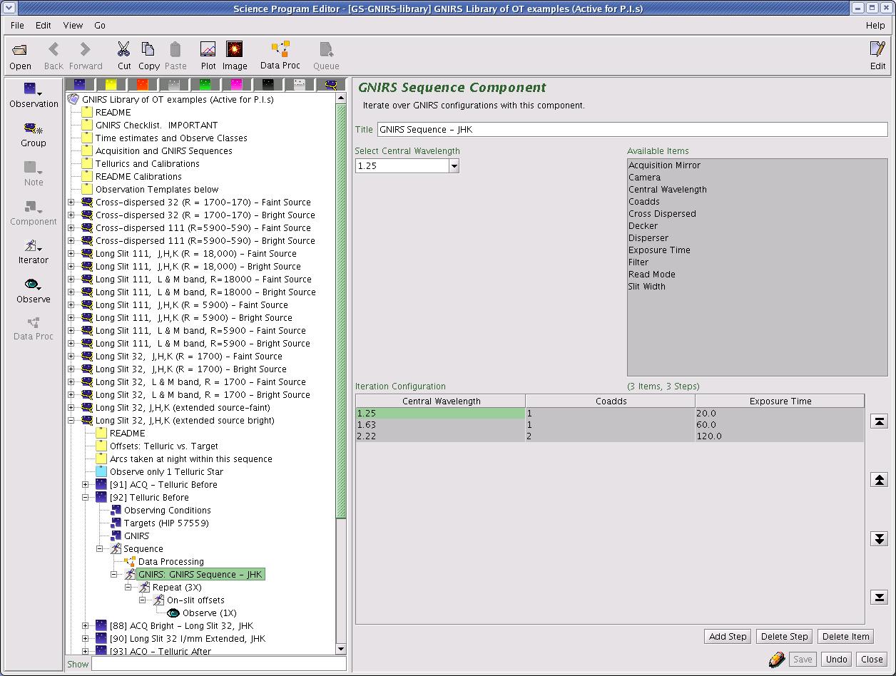
Set up an iteration sequence by building an Iteration Table. The table columns are items over which to iterate. In this example we are iterating over wavelengths, exposure time and coadds.  Table rows correspond to iterator steps. At run time, all the values in a row are set at once. Since there are two steps in this table, an observe element nested inside the GNIRS iterator would produce an observe command for each of the two wavelengths, using the specified integration times.  Note that every dark gray line is a step-- blank dark grey lines retain the values from preceding steps. 

GNIRS iterators are only required when the observation is stepping through different GNIRS configurations.  If you are iterating on GNIRS configurations and also dithering, the offset iterator would normally be nested inside the GNIRS iterator, and the observe command nested inside the offset iterator.  To repeat a dither pattern at each configuration, the repeat iterator must come between the GNIRS iterator and the offset iterator.  In the example above, the sequence repeats the dither pattern ("Obj-Sky") 3 times for each wavelength, taking 1 exposure at each dither position. See the science program structure for more details about nested iterators.

A good way to check your observing sequence is by clicking on the "Sequence" folder.  There one can view the sequence as a contiguous list of actions or as a timeline.

Offset Iterator

The offset iterator is a general iterator, common to all instruments.  With this iterator one can define the offset sequence to use for dithering on the sky.  Most infrared observations use some type of dithering to facilitate sky subtraction.  Typical examples are ABBA (two positions along the slit), and object-sky (on-source and off-source).  When using the long slit, the slit length is 99 arcsec, so one can dither along the slit at multiple positions for a point source (e.g., ABCDE), or use an ABBA sequence even for moderately extended objects.  However, in cross-dispersed mode, the slit is only 6.1 arcseconds in length.  For point sources, an ABBA sequence with a separation of 2.5-3.0 arcseconds will work; if a larger separation is required, an on-source/off-source (object-sky) sequence will be needed.  A separation of 2 arcseconds is possible  if very good image quality (<0.5arcsecs) has been requested.  Refer to the Observing Strategies page for more on dithering techniques.  When defining offsets, remember that "q" is along the slit (or IFU slice) and "p" is perpendicular to the slit (or IFU slice), always (regardless of instrument orientation).  One can check the offset positions with the position editor.

Acquisition Observations

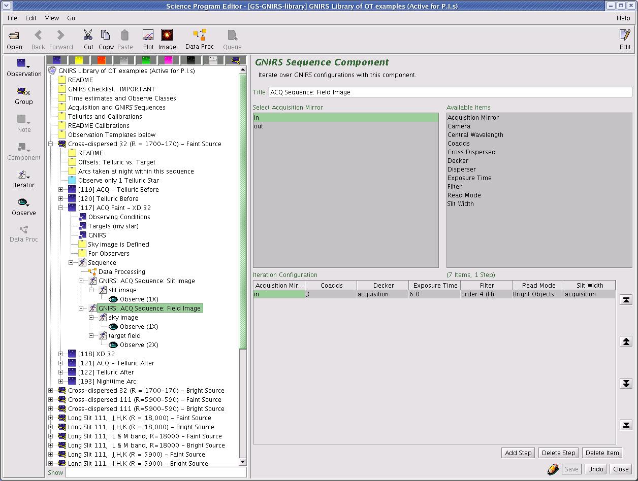
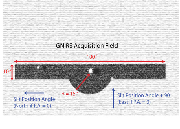
Acquisition is defined in a separate observation from the science observation. This is done to prevent inadvertent changes to the science observation. Here we describe the mechanics of creating an acquisition observation in the OT.  Appropriate acquisition exposure times are tabulated here. The GNIRS acquistion field scale and orientation is shown here. The acquisition procedure is described more generally on the Observing Strategies page. 

The best method is to make a copy of your science observation and replace the sequence portion with an acquisition sequence (leaving target and other instrument information unchanged).  The recommended procedure is the following.

1. After defining your science observation, copy and paste it (without moving your cursor, the new obs. will appear directly above).
2. Change the observation name to start with "ACQ - " (followed by science name).
3. DELETE the science sequence inside the Sequence component in the new observation.
4. Paste an Acquisition sequence in its place. Use the appropriate template from the OT Library that is specific to your instrument configuration and star brightness (i.e. faint, bright, or telluric). DO NOT change the static component (so as to keep the grating and prism turrets from moving).
5. Add a NOTE if needed, to provide the observer with helpful information, or explain any exceptions to the standard procedure.
   

• Choose from one of the following OT example configurations below:
• Long slit 32, JHK extended
• Long Slit 32, J,H,K (R = 1700)
• Long Slit 111, J,H,K (R = 5900)
• Long Slit 111, J,H,K (R = 18,000)
• Cross-dispersed 32
• Cross-dispersed 111
• IFU R=1700
• IFU R=6000
• Long Slit 32, L & M band, R = 1700
• Long Slit 111, L & M band, R=5900
• Long Slit 111, L & M band, R=18000
• In each case above, pick the ACQ case that matches your object (i.e.)
• ACQ - Faint: Objects with H > 14mag (includes a sky image)
• ACQ - Bright: Objects with 11 < H < 14mag (no sky needed)
• ACQ - Telluric: Objects with H < 11 (no sky is needed)
• In the GNIRS static component (see image below), edit the following items to match your particular observing case:
• Slit width: see pull down menu for options
• Central wavelength: For XD32 cases, always use 1.65
• Position Angle: PA=0 is a North/South slit


 



• In the GNIRS ACQ Sequence: Field Image component component (see image below), edit the following items to match your particular observing case:
• Exposure Time & Coadds: check here for appropriate acquision times
An example of a faint object acquisition sequence from the OT library is shown below:


 



Below are some supplemental explanations of how things are configured in the OT examples above:
• These are the ONLY items that should be needed for acquisition.  If you feel you need something else, ask your NGO or Contact Scientist first.
• Blank, dark grey areas repeat the information above-- i.e., in this example there are 3 steps with step 3 being identical to step 2.
• The first step will duplicate information from the static component where available, AND VICE-VERSA-- entries in the first step here will change the static component!  (This is why we keep acq. observations separate.)
  
• Each item:
• acquisition Mirror: must be IN.  this is the only place in the OT that the acq. mirror can be specified.
• coadds: may not be needed; include if the coadds is different than 1 in the static component, or if coadds are desired, e.g., for long acq. images.
• decker: blank entry in the first step will pick up the correct decker from the static configuration (it doesn't fill in because the decker is not explicitly included in the static component); later steps use "acquisition" for full acquisition field of view (FOV).
• exposureTime: a few (3-5) seconds is sufficient to image the slit; other exposure times depend on the object (see acquisition exposure times table).
• filter:standard acquisition is done with the H filter to maximize contrast between sky and object.  Other filters can be used, but will require different exposure times, and please alert the observer with a note.  Changing the filter here does NOT move the grating.  The "H2:2.12um" and "PAH:3.3um" filters are narrowband filters used exclusively for target acquisition.  These should be used to reduce throughput (for very bright targets, or L-band acquisition), or for specialized acquisition of a narrowband feature at one of these wavelengths.  In general, acquisition of objects brighter than ~10th magnitude (such as tellurics) should use the "H2" filter to minimize saturation.  If using the H2 filter, the slit should be imaged first with the H filter (step 1), the the H2 filter should be inserted in the subsequent steps for viewing the object.
  
• slitWidth: the first step picks up the slitWidth from the static component (to measure slit); later steps use "acquisition" for full FOV.  
• For simple acquisitions, these 3 steps are sufficient.  For sky subtraction, use the faint object acquisition sequence, which includes the offset to the sky position.  If a potentially difficult acquisition is anticipated, add a few more.  It does no harm to have more steps than needed, only those needed will be used.
• If desired, a final step can be added to re-insert the slit and decker and image the object through the slit.  The slit is repeatable to <0.5pixel and the decker to ~1 pixel.  (The acquisition mirror is only repeatable to a few pixels, which is why the slit is re-measured for each acquisition.)
• Do NOT include an offset iterator for offsetting to reference targets for "blind" acquisitions.  This will be handled by the observer.

---

Calibration Observations

PIs are required to specify all calibrations, including baseline calibrations, in their Phase II OT file. For baseline calibrations, this means "before" and "after" telluric standards and GCAL flats and arcs. These observations may be executed within the program or from a "general use" calibration program, but in either case will be charged as baseline. Calibrations in addition to the baseline set will be charged to the program, unless they can be executed in the afternoon (e.g., darks, twilight flats). See the Baseline Calibrations and Observing Strategies pages for more information. GNIRS flats and arcs are taken with the Gemini Calibration unit (GCAL). Flats and arcs that are taken with the data (i.e., without changing the instrument configuration) can be embedded inside the science or telluric observation.  The "Observe Class"must be set properly to ensure that the time accounting and proprietary period for baseline calibrations are handled correctly.  Calibration observations that are not executed within the science program, such as cross-dispersed flats, should be defined as separate observations that are executed separately from the science observations (these have Observe Class = "Daytime Calibration").  XD flats must be executed at the end of the night; IFU flats must be taken with the science data; all other flats can be taken separately or with the data, at the PI's discretion (see the GNIRS GCAL configurations page for more information.)


The OT calibration library includes typical GCAL calibrations for most common configurations. Duplicate copies of calibration observations are not required, but there must be one observation for each instrument configuration requested.  Exposure times and proper GCAL lamps/filters may need to be adjusted from the examples depending on the wavelength and slit width being used.  Proper GCAL/GNIRS configurations are available.


Telluric standards should be defined as a normal science observation would be-- including an acquisition observation and the desired offset sequence.  The only difference is the "Observe Class" which should be set to "Nighttime Partner Calibration" for baseline standards, or "Nighttime Program Calibration" for special/additional calibrations.

See Observing Strategies pages for more information.





---

Last update August 30, 2006; G. Doppmann