This page contains useful information for configuring F2 observations which should help reduce the number of iterations on the Phase II file between the PI and the NGO. It also contains an overview of the required OT observations and components for programs of different types. Before submitting your Phase II program to Gemini, use the F2 Phase II checklist to eliminate common mistakes.
Contents
- F2 Templates
- Required Observations and Components
- Overheads
- Imaging
- Long-slit
- Standard Stars
- Telluric Stars
- Observations split over several nights
- Observing Conditions
F2 Templates
Initially each program contains a template set of observations based on the examples of the OT instrument libraries. The PI should apply these templates to the observations. Please follow this template link with updated template information.
Required OT observations and components
For each type of program, there are different requirements to which OT observations and components the user has to define in the Phase II. The table below gives an overview over the requirements. "Required" means that a Phase II will not be accepted without this type of observation or component being defined. "As needed" means that the user can add this type of observation or component as needed by the science goals of the program. Use the F2 OT library as a source of template and example observations.
Ar arcs mixed with the science data, i.e. taken at night, and any special standard stars are charged towards the program's allocated time. Baseline standard stars, telluric stars, GCAL flats, twilight flats, baseline Ar arcs, and mask images are not charged (see the NIR Baseline Calibrations for more details). The time for the acquisition observations is already included in the science observation overhead. No additional time is charged. However, the acquisition observations have to be defined as separate observations in the Phase II.
Each "Observe" command is given an Observe Class (see more details about Classes).
The details of each of the required observations and components are explained in the sections below.
|
Observation or Component |
Program Type | Class | ||
| Imaging (details) Pre-imaging for MOS |
MOS (details) | Longslit (details) | ||
| Science Obs. | Required | Required | Required | Science |
| Offset Comp. | As needed | As needed | As needed | N/A |
| GCAL flats | Do not add | Required, one per 2h observation Mix w/ science |
Required, one per 2h observation Mix w/ science |
Nighttime Partner Calibration |
| Twilight flats | As needed Separate observation |
As needed Separate observation |
As needed Separate observation |
Daytime Calibration |
| Ar arcs | N/A |
Required, one per 2h observation |
Required, one per 2h observation Mix w/ science |
Nighttime Partner Calibration |
| Charged if more than one mixed w/ science | Charged if more than one mixed w/ science | Nighttime Program Calibration |
||
| Acquisition Obs. | N/A | Required Separate observation |
Required Separate observation |
Acquisition |
| If for telluric or standard | If for telluric or standard | Acquisition Calibration |
||
| Mask image | N/A | Required Separate observation |
N/A | Daytime Calibration |
| Telluric stars | N/A | Required, one per 2h observation | Required, one per 2h observation | Partner Calibration |
| Standard stars | As needed Separate imaging observation |
As needed Separate longslit observation Follow requirements for longslit |
As needed Separate longslit observation Follow requirements for longslit |
Nighttime Program Calibration |
Calculation of overheads
Detailed information about overheads for acquisitions (and re-acquisitions), as well as readout and configuration times can be found on the Overheads page. PIs can now use the calculated planned execution times in the OT as reasonable approximations of the actual time that will be required, with the exception that reacquisitions must be included when integrations times are long. If you do not take this into consideration, it is likely that your Phase II will be overfull. Gemini queue observers will stop executing your program when the allocated time has been depleted, regardless of whether or not there are still unexecuted observations.
If your observation classes are set correctly, the OT will not add any planned time for GCAL flats, twilight flats, baseline Ar arcs, telluric observations or other daytime calibrations (e.g. mask images and Darks). The support staff from your National Gemini Office and your Gemini Contact Scientist will work with you if you have questions about your OT calculated program execution time.
Program Organization
It is recommended that groups be used as much as possible to keep the Phase II organized. Some recommended organizational practices are:
- Group science observations with their associated acquisition observation(s).
- Organize all the time for long observations (more than 2 hours) into a single observation.
- Place the required telluric observation (both the before and after the science observation) in the same group as the science observations.
- Place all daytime calibrations in a folder called Calibrations
- Place time constraints (dates/times, temporal spacing of observations) within the Scheduling Note and within the Timing Windows under Observing Constraints.
- Group names within a program should be unique.
Imaging observations
All imaging observations should have a dither sequence. The choice of offset will depend on the nature of the science target such that small offsets are suggested for uncrowded and sparse fields and large offsets are recommended for extended and/or crowded fields. We include these two examples in the OT templates. In any event, we recommend that the first offset position should always have p=0, q=0.
GCAL imaging flat observations should be included in the Phase II. So please see this GCAL configurations table for recommended GCAL configurations and exposure times. At this point, we anticipate that the flats not listed will be dome flats. The Gemini staff would take care of preparing suitable dome flats if needed.
Long-slit observations
GCAL flats should be mixed with your science observations. For long observations, add one flat for every 1-2 hours of science exposure time. For observations shorter than one hour, add one flat. Make sure you get flats for all spectral configurations. GCAL flats within these guidelines have class 'Nighttime Partner Calibration' and are not charged to the program. Any additional GCAL flats should have class 'Nighttime Program Calibration' will be charged to the program. Refer to the GCAL configurations for recommended GCAL configurations and exposure times (examples are available in the F2 OT Library).
Ar arcs taken during the day as baseline calibrations. These calibrations are not charged to the program, but the PI has to define them in the Phase II. Define these observations as separate from the science observations and set the class to 'Daytime Calibration'. Make sure the instrument configuration matches the science observation. If you copy the science observation in order to edit it for the Ar arc, make sure to remove the guide star from the target component, remove any science exposures, and change the class. Arcs taken as part of a science longslit observations should have class 'Nighttime Program Calibration' and will be charged to the program. Refer to the for recommended GCAL configurations and exposure times. Also, complete examples are available in the F2 OT Library).
Acquisition observations need to be defined for each longslit target. No extra time is charged for these observations, as the overhead for setting up is already included in the science observation. However, the acquisition observations should be defined as separate observations in the Phase II. In general, we recommend to set up the acquisition sequences such that they include " sky " observations used to perform a sky subtraction during the nighttime acquisition. Only if the object is brighter than H=12 we consider that the " sky " observations are not needed. An acquisition observation for a longslit target should have the following instrument configuration:
Same target, guide star and PA as for the science observation
F2 filter closest to the spectroscopic filter
1) For Bright targets (H < 12):
Add a F2 sequence with at least 3 steps
Step1 - FPU: Imaging (none); Detector read mode: Bright Object; Exposure time: 5 sec
depending of the brightness of the target.
Step2 - FPU: Same longslit as for science; Detector read mode: Bright Object ;
Exposure: 10 sec. This step is used to measure the slit center and in the templates
includes a small offset. This offset shifts the target away from the slit center.
This is done so that light from the target does not interfere with the slit center measurement.
Step3 - FPU: Same longslit as for science; Detector read mode: Bright Object;
Exposure: 5 sec depending of the brightness of the target.
2) For faint sources (H > 12):
Add a F2 sequence with at least 5 steps
Step1 - FPU: Imaging (none); Detector read mode: Bright Object; Exposure time: 10 sec
depending of the brightness of the target; offsets: small offset in q for sky subtraction.
Step2 - FPU: Imaging (none); Detector read mode: Bright Object; Exposure time: 10 sec
depending of the brightness of the target; offsets: back to the target with p=0 and =0.
Step3 - FPU: Same longslit as for science; Detector read mode: Bright Object;
Exposure: 10 sec. This step is used to measure the slit center and in the templates
includes a small offset. This offset shifts the target away from the slit center.
This is done so that light from the target does not interfere with the slit center measurement.
Step4 - FPU: Same longslit as for science; Detector read mode: Bright Object;
Exposure: 10 sec depending of the brightness of the target; offsets: small offset
is applied in q. This observation will be used to perform a sky subtraction of the
next " on-source " observation.
Step5 - FPU: Same longslit as for science; Detector read mode: Bright Object;
Exposure: 10 sec depending of the brightness of the target.

Class: Acquisition
The science observations should include offsets. As it is the case for imaging, the choice of offset depends on the nature of the source. Thus, for sparse sources we recommend small offsets ( < 15 arcsec) whereas we recommend larger offsets (> 300 arcsec) for crowded and/or extended sources.
Twilight flatfields are only taken for longslit observations of extended targets. No extra time is charged for these observations. However, the twilight flatfields should be defined as separate observations in the Phase II. Make sure the instrument configuration matches the science observation. If you copy the science observation in order to edit it for the twilight flatfield, make sure to remove the guide star from the target component, then edit the science exposures to have only one exposure with 30sec exposure time and class 'Daytime Calibration'. If doing small wavelength dithers to fill in the chip gaps then only one wavelength setting will have a twilight flatfield taken, so you need to select the wavelength at which you want the twilight flatfield. If there are no twilight flats in the submitted Phase II for a longslit programs, it will be assumed that they are not needed.
Standard Stars
Imaging standards sufficient to obtain flux calibration at the 5% level are base calibrations and are taken by Gemini staff. If better calibration is needed then observations for additional standards must be included in the Phase II. The class should be 'Nighttime Program Calibration' and the time will be charged to the program. The PIs should also consider that given the F2 FOV at least a handful of " 2MASS " sources are probably included in the science observations.
Telluric standards used to cancel telluric (atmospheric) absorption features in the data are baseline calibration and are not charged to the program. Observations for these baseline telluric standard need to be defined in the Phase II including one observation that can be executed " before " and " after " the science observation. All telluric standards are taken in longslit mode using the same slit as for longslit science observation or the longslit closest in width to the width of the MOS slitlets. The observations needed are:
- Longslit acquisition with class 'Acquisition Calibration.' The longslit acquisition sequence for all telluric stars use the Bright Object read mode to image the field, measure the slit center, and to confirm if the target is within the slit.
- Spectroscopic observation with class 'Nighttime Partner Calibration'. Please select an exposure time long enough to obtain good signal-to-noise (i.e., 120 seconds). For longslit the instrument configuration should match the science observations.
- Daytime arcs with class 'Daytime Calibration'. All other guidelines for daytime arcs apply.
Additional spectroscopic standards --- absolute flux standards, velocity standards, line-strength standards, etc.--- must also be defined. If absolute flux calibration is desired then the 8-pix longslit should be used.
The guidelines are the same as for normal longslit observations except that the classes for the on-sky observes should be 'Nighttime Program Calibration'. The associated acquisition observations should have class 'Acquisition' and any GCAL flats are still 'Nighttime Partner Calibration'. The time will be charged to the program. Daytime arcs are always 'Daytime Calibration' and are not charged.
Observations that will be split over several nights
Some observations cannot be completed within one night and therefore will require multiple acquisitions. Exactly how such an observation will be split in several observations over several nights will normally be determined by the Gemini Staff at the time of scheduling the night's observations (see the overheads page for guidelines). The user should define such observations as one observation, and add a comment to explain which assumptions were made about the number of reacquisitions and the resulting overheads.
Observing conditions
The observing conditions are specified as percentiles in image quality, cloud cover, sky background (and water vapor). Refer to the observing conditions page for details about the meaning of these percentiles. If the percentiles do not give sufficient information to the queue observer about the observing conditions required for a given observation, the user should add a comment to the observation detailing the observing conditions, e.g. "Need fwhm better than 0.75 arcsec in r". Such comments cannot be used to request better observing conditions than approved by the time allocation process.
Baseline calibrations
NIR Baseline calibrations that are not specifically mentioned above should not be included in the Phase II programs prepared by the users.
MOS observations
Programs that contain MOS observations require masks designed from F2 pre-imaging taken for all separate fields. PIs with MOS programs are encouraged to submit designs as soon as possible.
MOS programs should contain the final Phase II information for the pre-imaging observations when it is first submitted. The MOS observations should also be included in the program. Small adjustments to the MOS observations are allowed when the mask design has been done. However, the pointing and PA of your target cannot be changed between the pre-imaging and the MOS observations. PIs with MOS programs will be contacted by Gemini when the pre-imaging data is available. Revised Phase II MOS programs and mask designs should be submitted asap. See mask deadlines (linked from the relevant semester's OT instructions page) for Classical runs. Mask designs should be submitted directly through the OT, instructions will be sent to you when your pre-imaging is available.
PIs with pre-imaging from previous semesters should use the mask naming scheme (below) for their current program. Upload the original pre-imaging through the OT so that masks can be checked. Please also include a note listing the previous program number.
The focal plane unit for the MOS observations should be specified as Custom Mask MDF, and the field for the name should contain your program ID and a running number for the mask within the program, e.g. for program GN-2014A-Q-20 the mask names should be GN2014AQ020-01 and GN2014AQ020-02 for the first and the 2nd mask, respectively. Note the leading zero on the program ID and mask numbers.
The total time used for both pre-imaging and MOS observations must not exceed the allocated time.
It is recommended that pre-imaging observations are dithered by 5 arcsec in both directions, e.g. 4 exposures in a square pattern with size 5 arcsec will work ok. Pre-imaging exposures should be taken in the broad band filter closest to the central wavelength coverage of the MOS observations.
GCAL flats should be mixed with your science MOS observations. For long observations, add one flat for every 1-2 hours of science exposure time (it is important to take GCALflats frequently for spectral observations at long wavelengths because of fringing, and less critical if observing in the blue). For observations shorter than one hour, add one flat. Make sure you get flats for all spectral configurations. GCAL flats within these guidelines have class 'Nighttime Partner Calibration' and are not charged to the program. Any additional GCAL flats should have class 'Nighttime Program Calibration' and will be charged to the program.
Ar arcs taken during the day are baseline calibrations. These calibrations are not charged to the program, but the PI has to define them in the Phase II. Define these observations as separate from the science observations and set the class to 'Daytime Calibration'. Make sure the instrument configuration matches the science observation. If you copy the science observation in order to edit it for the Ar arc, make sure to remove the guide star from the target component, remove any science exposures, and change the class. Arcs taken as part of a science MOS observations should have class 'Nighttime Program Calibration' and will be charged to the program. Refer to GCAL configurations for recommended GCAL configurations and exposure times (examples are available in the F2 OT Library).
Mask images are taken of all MOS masks before they are used for science. These calibrations are not charged to the program, but the PI has to define them in the Phase II. Define these observations as separate from the science observations. The instrument configuration should be as follows:
No guide star
J filter
Detector: Bright Object read mode
Class: Daytime Calibration
Define a GCAL flat using the appropriate information
from the following webpage.
For a complete example see the F2 OT Library.
Acquisition observations need to be defined for each MOS mask. No extra time is charged for these observations, as the overhead for setting up is already included in the science observation. However, the acquisition observations should be defined as separate observations in the Phase II. An acquisition observation for a MOS mask should have the following instrument configuration:
Same target, guide star and PA as for the science observation
F2 filter closest to the wavelength setting used
FPU should be Custom MDF mask and the same mask as for the science observation
Exposure time: 30-90 sec depending on the brightness of the acquisition stars
Detector: Bright Object read mode
Add an "observe", and edit it to show 4 exposures with class Acquisition
Broad band filters cannot be used for MOS acquisitions. Narrow band filters should in general not be used for MOS acquisitions. See also the example in the F2 OT Library.
Overheads
For calculation of specific system overheads where these are critical to your observing program (for example time-resolved observations), the detailed information on this page may be used. The detailed overhead information is also useful for the Phase II planning of your observing program. The various overheads can be broken into the following categories:
- Telescope setup time
- FLAMINGOS-2 configuration time
- Readout time
- DHS time
- Telescope offsetting time
- Calibrations
Telescope setup (acquisition) time
The setup times below include slewing to a new target, starting guiding, and accurately centering objects on slits (if appropriate).
| FLAMINGOS-2 mode | Config Time |
|---|---|
| Imaging | 6 minutes* |
| Long slit Observations | 20 minutes |
| MOS Obsevations | 30 minutes |
* overhead when using the PWFS2 guiding.
Applicants for FLAMINGOS-2 time should allow for one acquisition for approximately every 2 hours observed (including overheads and calibrations). Shorter observations may also be split in order to accommodate them in the queue planning.
FLAMINGOS-2 configuration times
Below are listed approximate configuration times for various components within FLAMINGOS-2 (the exact times depend on the details of the positions between which a particular component is being moved). It is possible to reconfigure FLAMINGOS-2 while slewing to a new target, but it is not currently possible to reconfigure FLAMINGOS-2 while reading out the detector. This is a limitation of the current software that is used to execute sequences.
| FLAMINGOS-2 component | Config Time |
|---|---|
| Filter change | ~50 sec |
| Grating change | ~40 sec |
| Mask move in or out | ~100 sec |
Readout times
Below are listed the overheads associated with reading out the array for both readmodes: a single CDS pair and for the correlated multiple sample (CMS) mode. The total readout time for the multi-read mode depends upon the number of reads (nreads); thus for 8 reads, the readout overhead is 20 sec. At present it is not possible to reconfigure FLAMINGOS-2, dither the telescope position or begin setup on the next target during readout.
| Read Mode | Time |
|---|---|
| CDS pair | 8 sec |
| CMS reads | 8 + (nreads*1.5) sec |
DHS Write times
The Data Handling System adds 7 seconds of overhead per frame to be saved. For long series of short exposures (e.g. deep imaging), this overhead becomes significant and must be taken into account.
Telescope offsetting time
The time to offset the telescope as part of a dither sequence is currently approximately 5-10s (from the time of turning off guiding at one position to guiding at the next position). At present it is not possible to offset the telescope while reading out the detector when these operations are part of a sequence.
Configuration for Calibrations
A portion of the overhead for taking calibrations is the time it takes to move the science fold mirror, which sends the beam either from the sky or from GCAL into FLAMINGOS-2. Again, when using the sequence executor to run sequences, this move cannot be done while reading out the detector array.
With FLAMINGOS-2 on side port 5, the relevant science fold moves take about 30 seconds each.
OT details
The FLAMINGOS-2 team strongly recommends that PIs read this section and also that they start from the automatically-generated OT templates for FLAMINGOS-2 OT library when preparing F2 observations. The library contains detailed instructions for customising the template observations: changing targets, standard stars, slit widths, etc. This web page is intended to explain the various OT components in depth:
After creating your FLAMINGOS-2 observations, please check the Checklist. If you still have questions, submit a HelpDesk query.
The FLAMINGOS-2 Static Component
Adding a F2 component to an existing observation, or adding a "F2 Observation" gives access to the FLAMINGOS-2 static component. The F2 component is used to define the basic F2 configuration and looks like this:
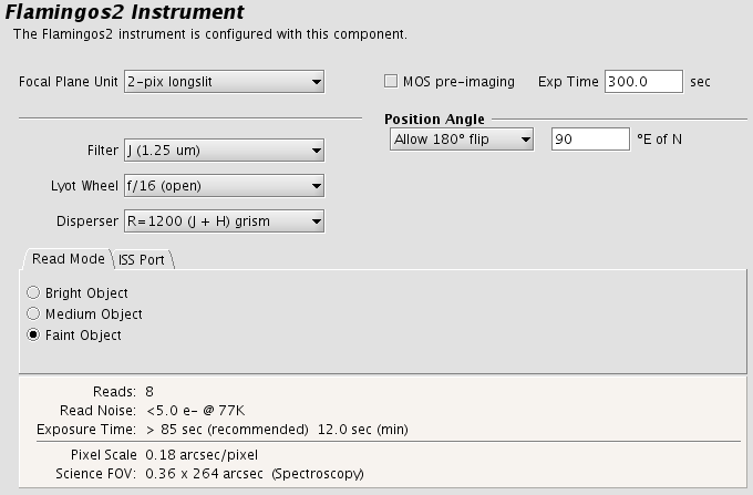
The available items are:
Select a suitable focal plane unit
Choice of one of the built-in focal plane units is made by clicking on the pull down lists (i.e. the down-pointing arrows) and selecting the desired unit. The built-in focal plane units included various longslits and calibration pinhole masks. For imaging, the focal plane unit should be set to "Imaging (none)". For MOS observations select the " Custom Mask" option.
Pre-imaging check box
If the observation is an image that will be used for a MOS design then please put a check mark on this check box.
Filter
The filter is chosen by clicking on the pull down list (i.e. the down-pointing arrow) and selecting the desired filter. The filter names are listed on the F2 filter pages (ignore the 5 character Gemini reference label). In spectroscopic mode, select the suitable filter for defining the spectral region of interest based on the desired spectral resolution (choise of grism as shown in the Grisms pages). A filter is always needed and the " Open " is not allowed. The filters JH and HK should not be used for broad-band imaging. The filter Y should not be used in spectroscopy mode.
Lyot Wheel
The LW position is chosen by clicking on the pull down list (i.e. the down-pointing arrow) and selecting the desired Lyot setting. The only option currently available for science observations is " f/16 (open) ". The other options are for engineering and future applications only.
Disperser
The choice of grism (for spectroscopy) or None (for imaging) is made by clicking on the pull down lists (i.e. the down-pointing arrows) and selecting the desired item. The grism names match those listed on the Grisms pages. If a grisms is chosen, a filter should also be chosen to provide the desired spectral coverage and resolution (see the Grisms pages for the available options).
Setting the position angle
The facility Cassegrain Rotator can rotate the instrument to any desired angle. The angle (in conventional astronomical notation of degrees east of north) is set by typing in the "Position Angle" entry box. The view of the science field in the position editor will reflect the selected angle. Alternatively the angle may be set or adjusted in the position editor itself by interactively rotating the science field. Select "Fixed" for a fixed position angle or "Allow 180o flip" to allow for a +/- 180 degree change when automatically selecting a guide star.
Users may also elect to use the average parallactic angle in order to minimize the effects of atmospheric differential refraction. This is recommended for long-slit observations where the position angle is otherwise unconstrained. When the"Average parallactic" option is selected, the nighttime observer will use the "Set To" drop-down menu to calculate the airmass-weighted mean parallactic angle. It is recommended that PIs set the PA to 90 for observations using the average parallactic angle and verify that a guide star is available. If no guide star is available with the OIWFS, the default guider should be changed to PWFS2, keeping in mind that flexure may require reacquisitions for observations longer than ~45 minutes. Note that the average parallactic angle option is only available for longslit observations.
Setting the exposure time
The exposure time is set typing the number of seconds in the "Exp Time" field. The exposure time depends on the chosen " Read Mode ". This choice defines the minimum acceptable exposure time.
Setting the read mode
There are 3 preset read modes. Each mode has a different read noise and overhead defined by the number of Correlated Multi samplings needed. The Bright Object mode is for bright objects and consists of one CDS read. Medium Object mode is an intermediate setting and consists of four CDS reads. The Faint Object mode is for the faintest objects and offers a low read noise and 8 CDS reads. Due to hardware clocking limitations Faint (Medium) Object mode can be set only for exposure times longer than 85 (21) seconds.
Short exposures should always be set to bright mode readout (i.e. 1 CDS read). A common source of time loss during the observation is a sequence which has the Flamingos-2 static component defined for faint (or medium) brightness object because the first exposure is longer than 85 (or 21) seconds, and somewhere in the middle of the sequence a shorter exposure is requested. This fault yields the detector controller unresponsive. If mixed readout modes are necessary in the same sequence, then specify the corresponding readout mode for each step in the sequence.
Selecting the ISS port
The location of the F2 OIWFS patrol field on the sky depends on which ISS port on the telescope has F2 mounted. Normally F2 is mounted on the "side-looking" ISS port. The OT has this selection as its default. It is important to make sure that the correct ISS port is selected for the current semester, since it affects whether the selected OIWFS guide star can be reached.
FLAMINGOS-2 Iterator
The F2 Iterator is a member of a class of instrument iterators. Each works exactly the same way, except that different options are presented depending upon the instrument. Below some of its features are shown in two examples. The first example is for imaging, the second example for longslit spectroscopy. The iteration sequence is set up by building an Iteration Table. The table columns are items over which to iterate.
The items that are available for inclusion in the iterator table are shown in the box in the upper right-hand corner of the F2 Sequence Components figures below. Selecting one of these items moves it into the table in its own column. Each cell of the table is selectable. The selected cell is highlighted green. When a cell is selected, the available options for its value are displayed in the box in the upper left-hand corner. For example, when a cell in the filter column is selected, the available filters are entered into the text box. When a cell in the exposure time column is picked, the upper left-hand corner displays a text box so that the number of seconds can be entered. When a cell in the "Custom MDF" column is picked, the upper left-hand corner displays a text box so that the mask MDF name will eventually be entered (not available yet).
Rows or columns may be added and removed at will. Rows (iteration steps) may be rearranged using the arrow buttons.
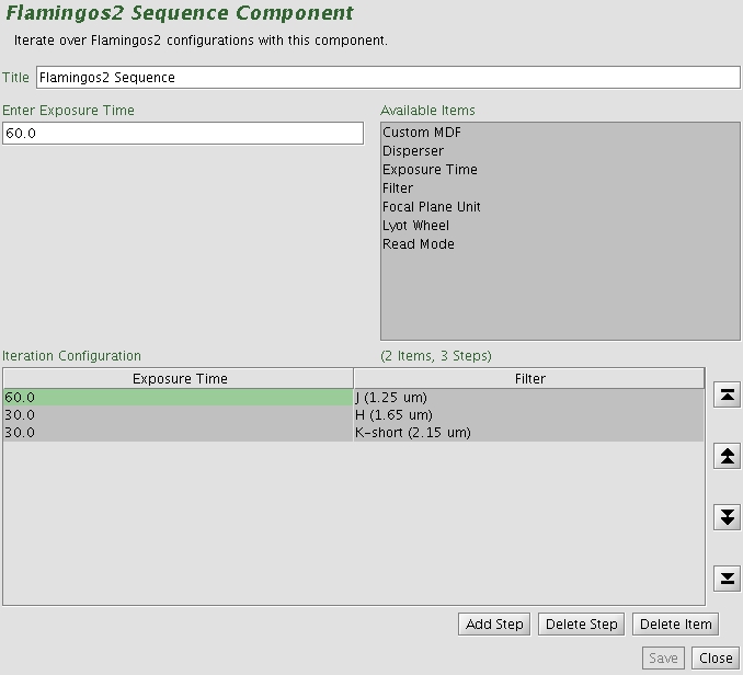
Example 1: F2 Iterator imaging example
 |
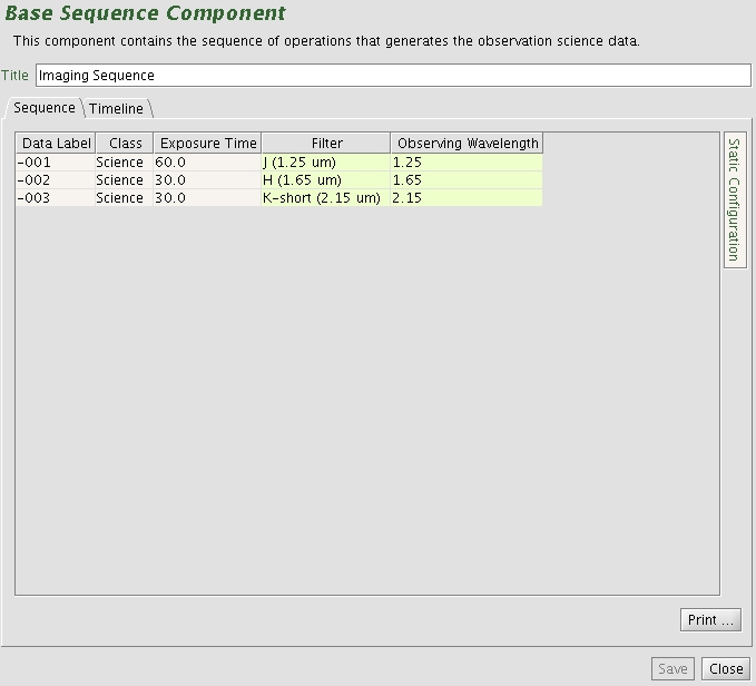 |
| F2 iterator example for imaging | The resulting sequence with one observe element and no offset iterator |
In this example the sequence iterates over filters and exposure times so there are two corresponding columns in the table. Table rows correspond to iterator steps. At run time, all the values in a row are set at once. Since there are three steps in this table, an observe element nested inside the F2 iterator would produce an observe command for each filter using the specified integration times.
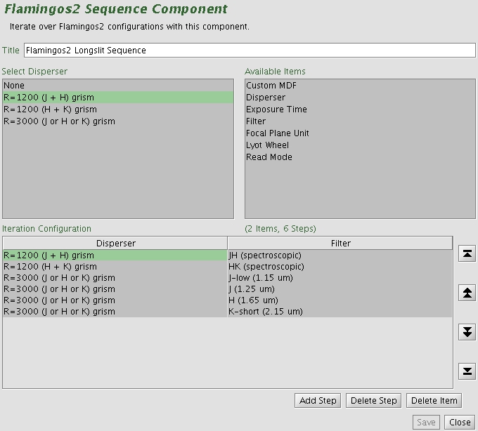
Example 2: F2 Iterator longslit spectroscopy example
 |
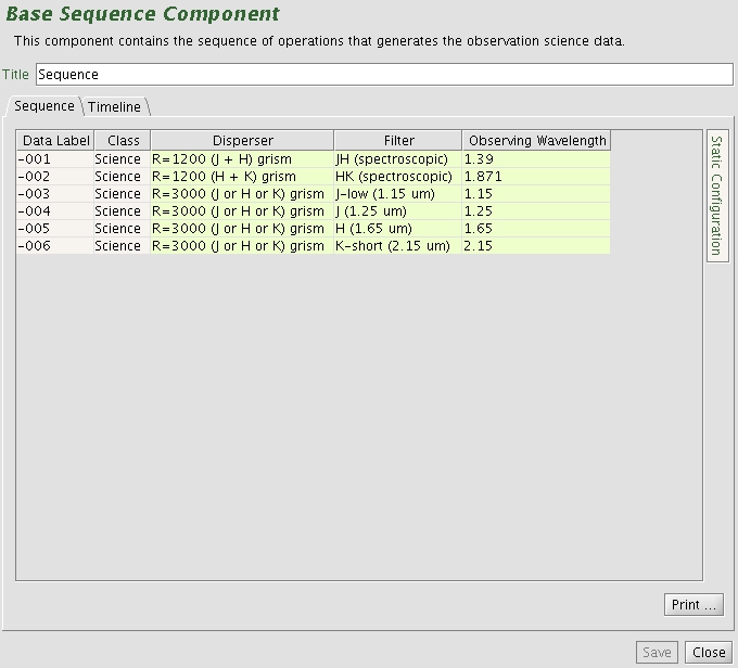 |
| F2 iterator example for longslit spectroscopy | The resulting sequence with one observe element and no offset iterator |
In this example the sequence iterates over all combinations of grism and filter for spectroscopy so there are two corresponding columns in the table. Table rows correspond to iterator steps. At run time, all the values in a row are set at once. Since there are six steps in this table, an observe element nested inside the F2 iterator would produce an observe command for each of six steps.
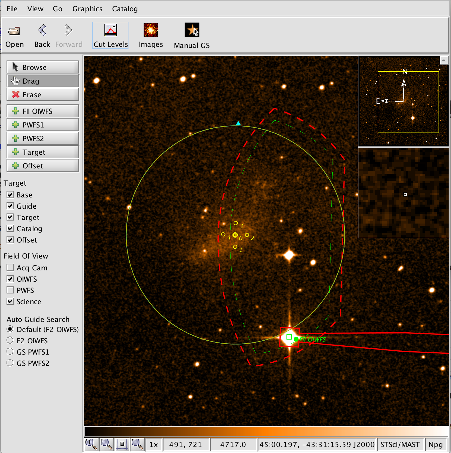
Viewing the FLAMINGOS-2 On-Instrument Wavefront Sensor Field
F2 is equipped with an on-instrument wavefront sensor (OIWFS). The region accessible to the OIWFS has an " asymmetric lens " shape, partly inside the imaging field of view, see the F2 OIWFS page for details. The OIWFS arm vignettes a small part of the field of view if a guide star inside the imaging field of view is chosen. The vignetting and the region accessible to OIWFS can be viewed with the position editor by using the Field of View: OIWFS item in the position editor menu bar. An example of this is shown in the figure below; the accessible patrol field is outlined with the red dashed line and the projected vignetting of the OIWFS is shown shaded in red. If multiple offsets are defined the green dashed line delineates the region within which valid guide stars may be selected, showing the intersection of the accessible patrol field for all the offset positions. The example is shown for F2 on the side-looking ISS port.
In cases where the science orientation is not critical, it is possible to rotate the instrument position angle to reach stars at other locations in the field.
Checklist for FLAMINGOS-2 Phase II (OT) programs
- General
- Have you selected appropriate templates from the F2 OT library? Have you gone through the checklist in the Top-level Program Overview note and included relevant standardized notes? Add notes with information about the program and acquisition that will make it easier for the observer. Try to use the standardized notes provided in the OT Library.
- In the F2 component, check that the best read mode has been selected for your science observation.
- Are the integration times reasonable? Minimum exposure times are defined by the read mode.
- F2 observation sequences that take longer than ~3 hours to execute will likely not be executed all on one night, and you must allow adequate time for re-acquisitions on subsequent nights when filling the allocated time. Have you read the details about the overhead calculations? Have you added a note explaining how many reacquisitions you have assumed for the calculation of the overheads? Taking the correct overheads into account, do your defined observations fit within the allocated observing time? Is there an appropriate mix of science exposures and baseline calibrations in the sequence?
- Have you checked Baseline Calibrations to see what is offered/required.
- Baseline arcs and flats should be set up using smartcals now. Choosing a flat (as observe element) within a science sequence will automatically set up a baseline nighttime partner calibration with an optimal exposure time. Choosing an arc within a science sequence will automatically set up the correct exposure time but these must be set to nighttime program calibration. Within a daytime arc sequence, this will be set up as daytime partner calibration. If you feel you need a different exposure time (to optimize counts within a particular region of the spectrum for example, use these tables as guidelines for recommended exposure times for GCAL Arcs and Flats. As of 2012B, arcs and flats configured manually will no longer be checked by either the NGO or Contact Scientist. Any time lost will be charged to the PI.
- Guide stars
- Are guide stars selected for the F2 OIWFS? The PWFS2 is not used with F2 in most cases. To choose a guide star for OIWFS, you can simply click on the Auto GS button in the OT position editor (with 'Allow +- 180deg change for guide star selection' chosen in the F2 component if appropriate). This will select an appropriate guide star for the specified observing conditions. Alternatively, the PI can still choose a guide star using the Manual GS button on the OT position editor. For manual guide stars, ensure that the guide star can be reached for the selected position angle, that the guide star is within the magnitude limits for the OIWFS, and that all guided offset positions can be reached. Check that the probe arm is visible and falls within the green box in the position editor. Fix any red offset positions. The UCAC3 catalog should be used whenever possible for choosing guide stars as the magnitudes are usually reliable.
- Ensure guide stars are stars and not galaxies.
- Calibrations
- Check that appropriate calibrations are included in the program. To see which baseline calibrations/standards are recommended, see Near-IR Calibrations.
- For twilight flats, make sure that the target component is left blank or excluded.
- If the PI requires calibrating standards beyond what is offered in the standard baseline calibrations, these must be defined, including a specific target, and time will be charged against the program for the observation. Observing class should be set to Nighttime Program Calibration. Baseline standards are set to partner calibration.
- Imaging
- Have you considered spatial dithers for imaging? These are normally needed to subtract the bright near-IR sky from the data.
- Baseline photometric standards should not be defined within the program. These baseline standards are already taken on each photometric night that imaging data is obtained. If the PI wishes to have more than one taken, or insists on having one taken with a program defined for CC70 conditions, then a program standard with target component will have to be defined in the program by the PI.
- Spectroscopy
- Have you considered spatial dithers for spectroscopy? These are normally needed to subtract the sky, avoid bad detector regions, and monitor the sky variations.
- Ensure that all the appropriate baseline calibrations (nighttime GCAL flats, twilight flats, daytime Ar, mask image obs [for MOS], and " before " and " after " telluric standards) and acquisition observations are included.
- Have you included the appropriate acquisition observations?
- If an observation includes an unusual or non-standard acquisition (eg. off-axis long-slit where the guide star cannot be accessed with the science target on-axis, blind offset acquisitions, MOS acquisitions with large initial offsets, etc), include the appropriate OT Library standardized note in the program. The text of the note can either describe the acquisition or point to other notes within the program. Using these standardized notes should minimize acquisition errors and would alert the observers about non-standard observations.
- BLIND OFFSETS: Use when targets are too faint to be acquired within 5 min of imaging.
- Make sure that a User1 target is defined with coordinates on the same astrometric system as the science
- Make sure the blind offset User1 star has a name, preferably something like 'Reference Star' or 'Blind offset star'
- Offset star should preferably be within 20 arcsec of the science target. The accuracy of blind offsetting is better than 0.1 arcsec for offsets less than 20 arcsec.
- For the blind offsetting to work, it is essential that the same guide star can be reached for the bright object and the science target.
- Include a note in the program to warn the observer of the non-standard acquisition.
- If your longslit spectroscopic observations involve complicated alignments, crowded fields, or targets fainter than about H=14.0 (eg. if the target is not obvious in the OT position editor with the 2MASS image loaded), you need to prepare finding charts. Such a finding chart should indicate the target/s and display the orientation (preferably North up and East to the left) and scale. Finding charts should be uploaded through the OT.
- If your program is a MOS program, have you defined any pre-imaging along with mask observations? You will get the chance to modify the MOS observations once you design your mask. However, the pointing and PA of your target cannot be changed between the pre-imaging and the MOS observations.
- For MOS programs, have you included the required daytime calibration mask image(s) .
- If your program is a MOS program, prepare yourself for the mask design by reading the MOS instructions in detail and installing the required software.
- Mask names must be in the correct format: ie for program GS-2014A-Q-20, the mask names should be GS2014AQ020-01 and GS2014AQ020-02 for the first and second mask, respectively.