Observation preparation | Gemini Observatory

This section contains instructions for configuring NIFS at phase II. It is organized as follows:

OT Details: How to configure NIFS in the Observing Tool (OT)
OT Library: A direct link to the example NIFS observations that should form the basis of your phase II submission (fetched from the database with keyword=123456, Program Reference=GN-NIFS-library)
Phase II instructions/deadlines for the new semester
Phase I/II Checklist: How to avoid common proposal and OT mistakes

The easiest way to develop a Phase II program is to use the predefined observations in the OT Library. The OT Library contains examples and templates of all typical Gemini observations and should be the basis of your phase II (the example best matching your desired observation can be copied and pasted into your program in the OT, and then modified to your requirements). The best practice is to use (or at least review) the library version for the current observing semester. This way, updates or changes to observation protocols will automatically be accounted for in new Phase II programs. Notes and descriptions appear directly in the library sequences to help observers understand how to best use the instruments.

Phase II submissions are required to contain spectroscopic acquisition sequences and all calibrations. Examples of observations with these calibrations included are also given in the OT Library.

Observing strategies

This page brings together information that might affect decisions on observing strategy in various NIFS observing modes, and provides guidelines/tips to maximize observing efficiency and avoid some common errors. The other NIFS web pages also give information about what to expect from the instrument. For information about actually setting up observations in the Observing Tool, please see the Observation Preparation section of these pages.

Here we describe briefly several factors that users may wish to take into account when designing their observing sequences:

Guiding

The type of guiding configuration you choose for your program has a significant impact on the quality of the data you will obtain. To assess the best strategy for your program you ought to have an estimate of: 1. the spatial profile for your source, 2. its brightness, 3. its proximity to bright point-sources.

With these details in hand please read: adaptive optics at GEMINI and guiding options with NIFS. To get (1) a feel for the possible corrections as a function of observed wavelength, and (2) a rough estimate of the relative importance of guiding star brightness and its proximity to your science target, you may find useful: those theoretical estimates of Strehl corrections obtained with Natural Guide Star (NGS) adaptive optics system

The Altair (AO) field of view is not a concentric circle around the NIFS field - it is a little off-centre and egg-shaped. If your guide star is close to the edge of the Altair field of view this may cause slight obscuration of the guide star, which can affect guiding. To gave some additional margin of uncertainty, you may wish to change the position angle to put the guide star a little more inside the accessible field for Altair.

If your source is large and extended, you might wish to set the acquisition for this source to use a blind offset. It is important that the star from which you can do the blind-offset is in the same guiding configuration as your science target.

If you choose SFO open loop guiding:

Please read this first: SFO open loop guiding .
If your target is extended it needs to be brighter than 16.5 mag in R. If it is a point source you can use this method for a source as faint as 18.5 mag. However, in that case you should have a back up guiding strategy, e.g. LGS + P1 or natural seeing.
In general SFO re-tuning takes less time than an acquisition but it depends of the magnitude of the SFO star and the magnitude of the galaxy nucleus. To minimize overheads plan two hour observation blocks with a SFO re-tuning in the middle. This works best for SFO star brighter than 12 mag and nucleus brighter than ~15.5 mag. Better corrections may be obtained by re-tuning every ~ 45 minutes.

Read Modes and Use of Multiple Coadds

In the OT the read mode is automatically set based on the length of the individual exposures. The OT will not dynamically change the read mode, but the template observations will have the read mode (and exposure time) set based on the source brightness. In particular:

IF K<=9 THEN Read Mode = Bright Object, Exposure Time=10
IF 9 < K<=13 THEN Read Mode = Medium Object, Exposure Time=80
IF K > 13 THEN Read Mode = Faint Object, Exposure Time=600

NIFS supports coadding which involves taking multiple exposures and writing the average to a single FITS file. The benefit is avoiding the overhead associated with writing multiple FITS files (8 seconds per file). The downside is that cosmic rays from each exposure will be inextricably merged, and of course, coadded exposures may not be dithered. Coadding is therefore most useful for programs which must take many short exposures to detect faint features without saturating bright objects.

Non standard central wavelengths

We have noticed that the grating is somewhat less reliable when using non-default central wavelengths. This is a feature of the mechanism control. For this reason, if the nominal wavelength range does suffice, it is recommended that you use it.

Observing Conditions

Dry observing conditions are typically only required when measuring spectral features in the wings of the atmospheric transmission windows. Please refer to this page for relevant plots at different wavelengths.

Fainter guide stars may require gray (SB80) or even dark (SB50) sky brightness conditions. Note, however, that constraining the sky brightness will reduce the probability of completing such observations as gray/dark time occurs less frequently and is in high demand because of competing optical programs which are sensitive to sky brightness.

Telluric

Given the strength and variability of sky lines in the IR it is important that telluric standards are observed at most every 2 hours, and preferably after each 1.5 hours of observations. In most cases, the time spent on tellurics are not charged to the program but to the partner country. However if more than one telluric is required for each 2 hours of observing time, those additional tellurics are charged to the program.

This link will help you find the right telluric given the coordinates of your source and the duration of the on-target observation.

Please check if your telluric is a double or if it may lead to saturation. NIFS's response becomes non-linear (~6%) at 38,000 and saturated at 48,000 ADU. For non-AO (P2) observations, the integrated flux is fairly similar to the AO integrated flux, but the peak flux on the detector at the peak of the PSF is easily a factor 10 lower. So with AO, the bright limit for NIFS is around K=5.
For P2, it is more like K=3. There are neutral density filters which can be used to bring down the flux if needed. They are not used very often, and their spectral signature is not well caracterised, so additional calibrations may be needed for those cases.
For P2 tellurics, it is recommended that you slightly increase the exposure time to compensate for the lower peak flux, but not longer than 30s. Going longer than 30s on tellurics (either AO or P2) is not efficient, and usually not needed - you can usually find a brighter hot star, perhaps by going to A1-2 type instead of A0.

Please use the integration time calculator (ITC) or the table below page to estimate the required exposure times for tellurics.

Estimated Exposure Times for Tellurics
Exposure Time per Frame (sec)	Observing Conditions
	IQ85/CC70	IQ85/CC50	IQ70/CC70	IQ70/CC50	IQ20/CC70	IQ20/CC50
5.3	K = 6.5 - 5 mag	K = 7.5 - 5 mag	K = 8 - 5 mag	K = 8 - 5 mag	K = 8.5 - 5.5 mag	K = 8.5 - 5.5 mag
10	K = 7.5 - 6 mag	K = 8.5 - 7 mag	K = 8.5 - 7 mag	K = 9.0 - 7 mag	K = 9.5 - 7.5 mag	K = 9.5 - 7.5 mag
15	K = 8 - 6.5 mag	K = 9 - 7 mag	K = 9 - 7 mag	K = 10 - 7.5 mag	K = 10 - 7.5 mag	K = 10 - 7.5 mag
20	K = 8.5 - 7 mag	K = 9 - 7 mag	K = 9.5 - 8 mag	K = 10 - 8.5 mag	K = 10 - 8.5 mag	K = 10.5 - 8.5 mag

Maximum Exposure Times and Saturation

The maximum exposure time you should use is set by several constraints:

(1) Saturation on the sky
(2) Saturation on the object
(3) Sky variations during a dither sequence

Individual exposures longer than 900 seconds are not recommended due to sky variations on those time scales.

Offsetting (Nodding, Dithering)

Small dithers e.g. 0.3" are encouraged to account for variations in spaxel sensitivity.

Infrared observations generally require background subtraction. Here are some guidelines:

For objects that fill the NIFS FOV, off-source sky observations are required. Depending on your guiding configuration and the size of your source you may have to set the guiding to "freeze" at sky position outside the guiding range of your guiding configuration.
Generally it is recommended to spend the same amount of time on object and on sky for best sky subtraction, and to have each science frame adjacent to a sky frame.
Cross-talk when observing bright sources H < 8 with fainter structure (e.g. observations of young stellar jets):
- "Cross-talk" is a smearing of flux along the IFU image slice that has the bright stellar PSF. This shows up as a brighter line of flux in the +/- y direction in the NIFS data cubes. Relatively speaking this is a small effect. However, it can decrease the S/N on faint emission if that emission happens to be aligned with this effect. The recommendation for such cases is that you rotate the NIFS field so that the jets are perpendicular and don't align with this flux smearing effect.

Understanding your PSF

There are several methods to estimate your PSF, several of those have been employed in refereed publications. Here we suggest the observational PSF that will facilitate the ideal PSF determination
- Distance between guide and PSF star should be the same as the distance between the guide and your Science target +/- 3"
- Magnitude of guide for the PSF observations should be the same as the magnitude of the guide for your Science +/- 0.5
- Position Angle PSF-Guide to PSF should be the same as position angle of Science target-guide to Science target +/- 20degrees.
- The declination of your PSF should be the same as that of the Science target +/- 5 degrees.
- You strive to achieve the same SNR for your PSF observation as you will for your Science star.

Coronagraphy Observing Strategies

R~5000 infrared IFU spectroscopy at AO resolutions using the 0."2 or 0."5 occulting disks for coronagraphic measurements is available. The best performance is achieved in the H and K bands. Coronagraphy can be carried out with or without ALTAIR's field lens, and with or without a NIFS OIWFS guide star. However, for best results, use of the field lens and OIWFS is recommended (OIWFS is currently not available). It is important to note that minimum of support is offered for the coronagraphy mode and the mode is better suited to users with previous experience with coronagraphic data and with coronagraphy observing strategies.

Overheads

Current estimates are that the overheads associated with each new science target (for target acquisition, telescope, WFS and instrument re-configuration etc) depend upon the guide configuration chosen for the observation.

Setup times for various observation types are:

Mode	Setup times
NIFS+PWFS2 (non-AO)	11 mins
NIFS+Altair-NGS	11 mins
NIFS+Altair-LGS	25 mins
NIFS OIWFS	add 5 mins
NIFS Coronagraphy	add 4 mins

Long observations may be split over several nights to better accommodate them in the queue. Please allow for one acquisition for every 2 hours of observing when calculating the time required for your project.

Acquiring with the coronograph requires some additional iterations during acquisition to ensure an accurate centering behind the occulting disk. Likewise, acquiring the OIWFS star incurs an additional overhead of approximately 5 minutes. These overheads are in addition to the baseline set-up time for a given guide configuration. For example, the assumed overhead for an NGS-AO coronographic observation including an OIWFS star (recommended) is 11+4+5 = 20 minutes.

Dithering overheads: 30s per dither step

For the small 3" x 3" FOV of NIFS, it will be necessary to dither the telescope off the science source to acquire a sky spectrum for nearly all observations (see examples in the OT Library).

For automated sequences of exposures (dither patterns) the estimated on-source efficiency is ~40%; (i.e. 60%; of the elapsed time is used for detector readout, telescope offsetting, WFS re-acquisition etc). This estimate is quite realistic for a typical target->sky->target->sky... observations.

Very short exposures will have lower efficiency because of the fixed overhead per image (up to 30 seconds for dithers). Longer exposures will have higher efficiency.

Readout overheads

Observations in the low noise readout modes incur higher overheads. Standard "bright object" readout requires 5 seconds per image, medium read mode is 21 seconds per image, and the "faint object" readmode, which provides the lowest 6e- readnoise, requires 85 seconds to read out each frame. Also, readout overheads accumulate for every coadd, so a "faint object" observation that has 8 coadds will have 8 x 85 = 680 seconds of readout overhead! This is not recommended. For optimal efficiency, it is best to chose a readmode based on the brightness of your target and the length of the individual exposures.

Readmode	read noise	readout time (per coadd)
Bright source	18 e-	5.3 sec
Medium source	9 e-	21.2 sec
Faint source	6 e-	84.9 sec

Grating change overhead: 65s

A new OT for 2006B CfP should have all the above NIFS overheads properly handled, then "Timeline" in the "Basic Sequence Component" should be close to the actual exection time (i.e., wall clock time).

The current OT assumes a fixed overhead (0.17 min = 10.2 sec) for all telescope & instrument setups. Actual times for some of these setups are quite off from the fixed overhead of 10.2 sec. Two main discrepancies are offsets (or dithering) and grating changes. For each dither position, overhead is ~30 sec (instead of 10.2 sec) and a grating change takes typically ~65 sec.
The "Planned Observing Time" value from the current OT includes only actual exposures plus the initial target setup time. It does not include any telescope and/or instrument overheads after the initial target setup. A true observing time can be obtained by adding up all items which appear in the "Timeline". To see this "Timeline", click sequence -> TimeLine.

NIFS in the Observing Tool

Like all Gemini facility instruments, NIFS is operated through the Gemini observing tool (OT). This page guides you through the main steps and considerations for configuring NIFS observations in the OT.

NIFS OT Basics
NIFS Component - Baseline configuration in the OT (filters, gratings, exposure times etc.)
NIFS Iterator Component - Defining observation sequences

NIFS OT Basics

If you are unfamiliar with the OT for NIFS, then the following information will introduce you to the basics. If you are familiar with the NIFS OT, then you might jump to the next section and start defining your phase II proposal. Basic information on the OT itself is available here.

NIFS observations are specified in a hierarchy of elements. The primary configuration component is the NIFS component. In this section we describe:

Suitable Grating and Filter Combinations
- Disperser central wavelength
- Non-standard central wavelengths
Focal Plane Mask
Position Angle
Controlling the Exposure Time
Selecting the appropriate Array Readout Mode

Since NIFS can be used in stand-alone mode or with AO-assisted observations when coupled with ALTAIR (NGS and LGS), we describe how to set up observations in the OT both with and without an AO-feed. It is also important to specify guide stars for Altair and possibly the peripheral wavefront sensor (PWFS2) or on-instrument wavefront sensor (OIWFS) which includes:

Stand-alone operation
- Specifying suitable guide stars for non-AO observations with NIFS
AO-assisted NIFS+ALTAIR observations
- Configuring the ALTAIR AO Component including setup for observations with the LGS
- Specifying appropriate guide stars for the AO correction (AOWFS) and flexure compensation , if appropriate (OIWFS)
- LGS and NGS specific information

Once NIFS has been correctly set-up the actual observation is defined in the NIFS Iterator Component. In this section we describe the elements of this iterator:

Instrument iterators
- Using a sequence of different grating settings
- Advice for long observations
- Checking the status and progress of the instrument with the "Sequence" tab
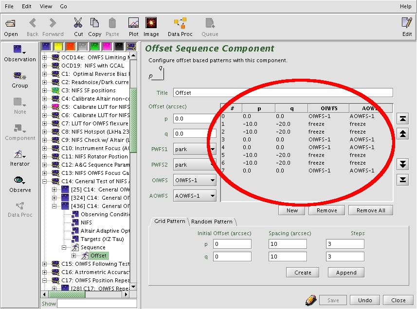
- Offsetting and dithering

Together with the information and examples given in the NIFS OT library, you should be able to configure your observations within the OT.

Please also refer to the general NIFS pages for further information on the instrument. Once you have completed your phase II, please see the NIFS checklist to verify the completed phase II program includes all of the items a PI needs to consider to get the best out of their observations.

NIFS Component

The detailed component editor for NIFS is accessed in the usual manner, by selecting the NIFS component in the science program, and is shown below:

NIFS OT Component

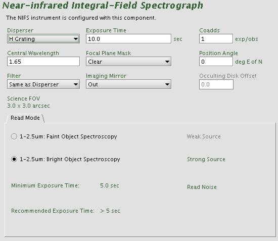
Selecting a grating, filter, central wavelength and focal plane mask

Typically, the grating for the observation is chosen first. NIFS has four gratings physically mounted in the dewar. Each default configuration of grating choice uses a dual blocking filter, one of Z-J, J-H, or H-K for Z and J, H, and K gratings, respectively. The grating/filter tables explain the proper combinations.

Once the grating is selected, the default central wavelength will automatically be entered into the NIFS component. NIFS covers essentially all of the associated photometric band in one shot, and the default settings (see grating/filter tables) are designed for this case.

If the filter is chosen as "Same as Disperser", then the appropriate default blocking filter is selected at the time of observation.

The instrument can be configured to modify these default grating settings by choosing a different central wavelength, these setting are described in grating/filter tables. This should not be necessary for most programs, however, at least three additional possibilities may be useful. One is to rotate the grating turret to shorter K band wavelengths to observe further into the telluric band near 1.9 um. Paschen alpha, for example, can be observed from Mauna Kea on dry nights. Similarly, one can observe at longer K band wavelengths.

The focal plane mask should be "Clear" for regular observations. For coronagraphy, several focal plane occulting masks are available for observations of bright targets with faint companions.

The "Imaging Mirror" should be "In" in the acquisition sequences if the target is faint as Kmag>13. Otherwise "Out.".

Controlling the exposure

The exposure time is set by clicking in the dialog box and typing the required number of seconds. Each occurrence of the observe element will cause N exposures to be taken and coadded in the instrument control system resulting in a single image written to disk. The value of N is set by typing an integer in the "coadds" window. The total integration time in each output image will be the "Exposure Time" times the number of coadds.

Setting the position angle

The facility Cassegrain Rotator can rotate the instrument to any desired position angle. The angle (in conventional astronomical notation of degrees east of north) is set by typing in the "position angle" box. The view of the science field in the position editor will reflect the selected angle. Alternatively the angle may be set or adjusted in the position editor itself by interactively rotating the science field.

Array readout mode

Choose either bright or faint object mode. Objects fainter than about K~10 should use the faint object mode. The array chacteristics given in green at the bottom of the OT screen will get updated when a different readmode is selected.

NIFS stand-alone (non-AO) mode

It is possible to use NIFS in stand-alone mode (without ALTAIR); please see the Guiding Options page for details. Guide corrections for non-AO NIFS observations are provided by the Peripheral Wavefront Sensor, PWFS2.

NIFS+ALTAIR: AO-assisted observations

To use NIFS with AO mode, an ALTAIR AO component should be included in your observations, and AO guide stars must be specified.

Altair AO Component

This component must be included in the observation only if NIFS is to be used with Altair.

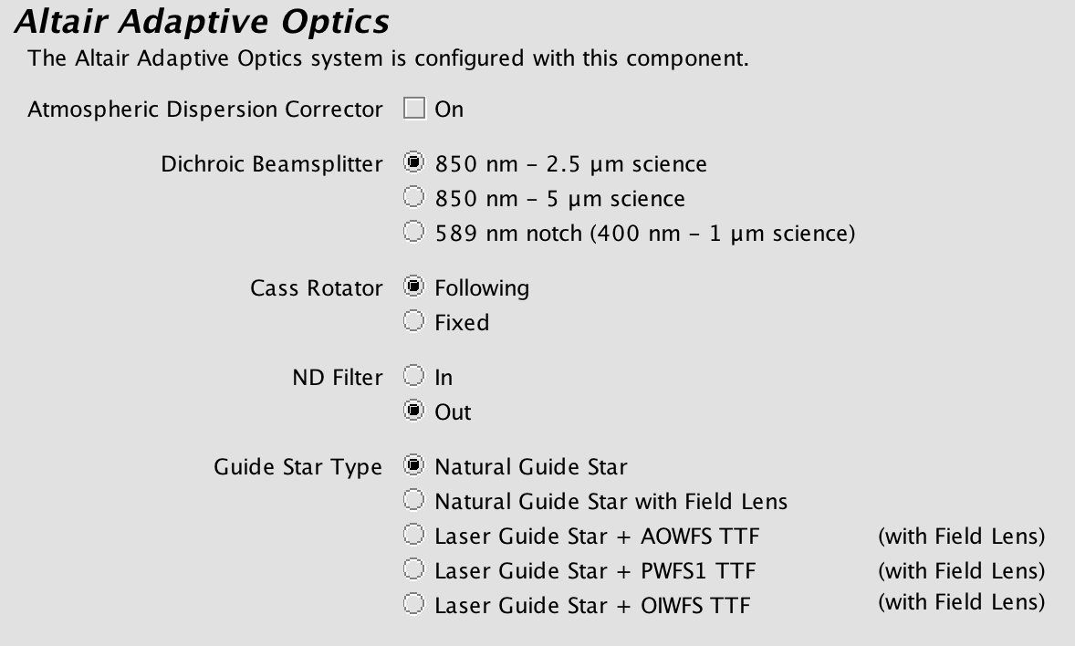
The component allows the observer to choose a dichroic for Altair. The 850 nm - 2.5 µm dichroic should be used with NIFS. Observers should choose the default "following" for the Cass Rotator to take out field rotation and keep objects fixed on the NIFS detector. The OT includes a selection for the Altair field lens.

Specifying AOWFS Stars and Guide Stars for NIFS

The Altair "AOWFS" star is specified in the targets section of the main observation as shown below. For on-source correction of the wavefront, the coordinates of the AOWFS star should be identical to the target coordinates (the Dist field should show "0").

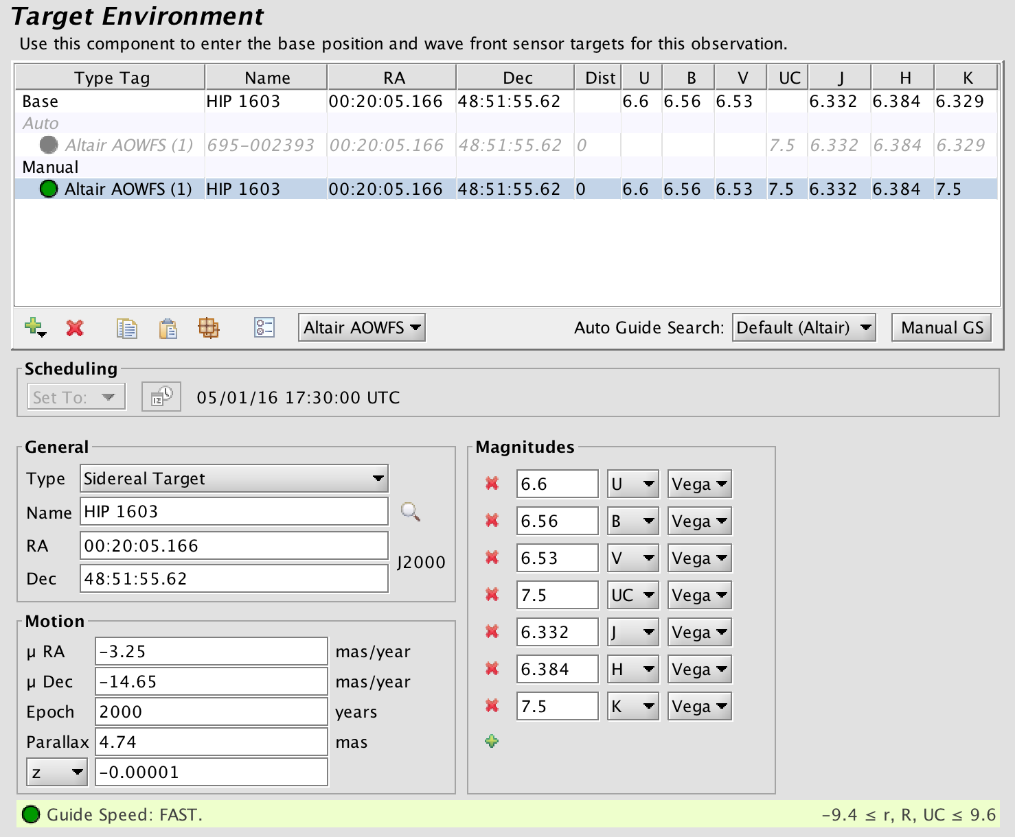
Information about the base position (i.e. the science object) and guide star(s) may be editied by clicking the appropriate line in the target table at the bottom and then editing the various fields through the text boxes above. Changing the type of target may be done using the "tag" pull down menu at the upper left.

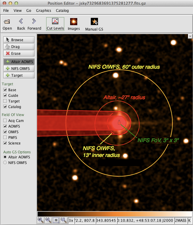
The OT will automatically select UCAC4 guide stars based on the instrument configuration and conditions. Details are given on the guide star selection help page. Manually-selected guide stars can be added (green +) or deleted (red X) manually. You can also use the Position Editor to query an image of the field and add stars interactively from the UCAC4 or PPMXL catalogs.

An example image field is shown below (from the position editor) with the science field (small green box) and WFS fields overlayed (red and yellow circles). The NIFS pickoff probe is outlined as well in red. The yellow circle is the OIWFS field and the red/green egg shape is the useful Altair field for wavefront correction. Since the AO fold mirror in the Cassegrain instrument cluster first sends the telescope beam to Altair, the Altair field is unvignetted. The NIFS science field pick off will vignette the OIWFS field as shown. If using Altair then the outer limit of the OIWFS field depends on the Altair field lens option and the display will update accordingly. The Cassegrain rotator may be adjusted (position angle) to access OIWFS guide stars which would otherwise be vignetted.

Things to remember or consider for choosing suitable NIFS guide stars:

All observations must have a guide star. This will usually mean at least an AOWFS star.
AOWFS stars should be as bright and close to the target as possible, and no further than ~27'' away. See the Altair pages for full details, or the NIFS guiding options page for a summary.
Always make sure to check that the selected observing conditions for cloud cover (CC) are consistent with the guide star brightness.The OIWFS can be used in combination with the AOWFS star for long observations where flexure between NIFS and Altair might be important. See the guiding options section for more details.

NIFS Coronagraphic Observations

Attenuation of light from the target will greatly depend on how well the object is aligned behind the coronagraph of choice. As a result, every coronagraphic observation should have a dedicated acquisition sequence. For good suppression of scattered light, your target should be aligned with the center to better than ~10% of diameter of the occulting disk. For an example of coronagraphic observation acquisition sequence, check coronagraphic observation samples in the OT Library for NIFS. The smaller the occulting disk, the longer it will take to get your object properly aligned behind the mask.

If your coronagraphic observation requires sky frames between target frames, we strongly recommend that you only use the larger, 0."5 occulting disk for your observations. When offsetting to sky, it is much more difficult to keep a target adequately centered to <0."02 behind the small 0."2 occulting disk. Using the 0."5 disk will result in less observing overhead because of target centering and will result in more efficient observations. For sky offsetting, your phase II file needs to set guide stars to the "freeze" state for your sky offset position. This means that you need to set AOWFS and OIWFS to "freeze" if you are observing with NIFS+Altair+OIWFS (see the example below).

NIFS Iterator Component

The NIFS Sequence Iterator is a member of a class of instrument iterators. Each works exactly the same way, except that different options are presented depending upon the instrument. Use this component to change the instrument configuration during the observation, for example, to repeat the same basic observation at two grating settings. For observations that take a significant amount of time (approximately greater than 1 hr) iterating the instrument configuration between multiple gratings is not a good idea. This is because observing conditions may change, calibrations need to be taken, or the queue operator will only have limited time on any given night to complete part of the observation. In this case, break up NIFS observation into a separate "Observation" and best practice is to cut and paste your observations and change the instrument configuration for each separate observation. This allows for more flexibility at the telescope. Short observations of bright targets are good candidates for an instrument configuration iterator.

Below we see a few of the iterator features in the right panel of the OT tool (the left panel shows multiple observations in the NIFS Library with the details of observation 1 shown):

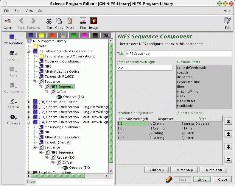
An iteration sequence ("NIFS Sequence" in the above image) is set by choosing "NIFS Sequence" from the "iterator" menu. The table columns in the "NIFS Sequence Component" are items over which to iterate. In this example we are iterating over gratings (and hence filters and central wavelengths which are not set automatically in this component) so there are three corresponding columns in the table. Table rows correspond to iterator steps. At run time, all the values in a row are set at once. Since there are four NIFS configuration steps in this observation and an offset iterator below (in this case with a five-point dither) an "observe" element would produce an observe command for each of four grating setups times the number of offsets (five), using the specified integration time, focal plane mask, etc. specified in the main NIFS component:

NIFS Sequence Table

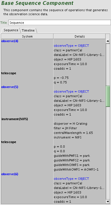
In the above figure, the iteration table shows parts of observe 4, 5, and 6 (of 20 total). The first five exposures are taken with the step 1 configuration (in this case the K grating) with the telescope dithering before each exposure (p, q offsets). After step 5, the instrument is re-configured with the H grating for the next five offset exposures.

Rows or columns may be added and removed at will. Rows (iteration steps) may be rearranged using the arrow buttons. Rows will be added or removed by clicking "Ad Step" or "Delete Step" buttons, and columns can be deleted by clicking "Delete Item". Adding column can be done by selecting one from the "Available Items" box.

NIFS Phase II (OT) Checklist

To speed up acceptance of your phase II file so that your program can be scheduled, observed, you may wish to consider the following checklist. When setting up your program in the OT, please also consult the NIFS observing strategies section and download and look at the example observations in the OT libraries.

There is a general OT/Phase II checklist that may be useful to consult.

Here is the NIFS checklist for Phase II, of which most, but not all, are NIFS-specific. For more information on most of these questions, please consult the NIFS OT Details pages along with the general instrument pages.

Guide stars:
- Did you read those pages: adaptive optics at GEMINI and guiding options with NIFS?
- Did you choose only one guide star (the brightest in guider FOV) per wavefront sensor you are using?
- Is the selected guide star(s) brighter than the guiding limit? If not the OT will complain. You need to address this complaint.
- Is the selected guide star(s) within the guide separation limit? If not the OT will complain. You need to address this complaint.
- Is the guide star a double? If so pick another.
- Is the Altair lens in?
- Does your guide star needs SB50/SB80 conditions? Please see the observing strategy page.
- If your observations involve blind offsetting, please add notes in the OT that re-acquisitions are necessary every 45min.
- Are you guiding with LGS + P1? Since there is no flexure model in place, we do not support blind offset observations where the target is not visible in individual science exposures. Please see this page: LGS + P1
- Is the guiding for standards set up properly? Most standards should use NGS, unless you wish to use the standard as PSF and want to observe in the same configuration as the science. Please see NIFS observing strategies.
Instrument configuration:
- Did you choose an appropriate grating and filter?
- Did you choose an appropriate readout mode?
- Are the focal plane mask and imaging mirror set correctly (for normal observation, FPM='clear' and Mirror='out')?
- Do you wish to set the position angle ? Please refer to the observing strategy page.
- Does your program require blank sky frames (i.e. your source fills the IFU FOV). If so, are sky offsets set up correctly and is offsetting going to a blank IFU field?
- Do you need multiple coadds? Please refer to the observing strategy page.
Acquisition Sequences:
- Did you include a finder chart? It is often needed, and it never hurts. Did you follow the guidelines for making your finder chart?
- Is the imaging mirror necessary for the acquisition? (i.e., target K mag > 13?)
- If the imaging mirror is needed, did you include a sky offset in the acquisition sequence?
- For the sky-offset steps, did you turn guiding off if the sky frame is not within the guiding limit?

Calibrations:
- Are GCAL arc exposures merged with the science for wavelength calibration? It is recommended that you obtain at least 1 arc per 2 hours of observations.
- Are the appropriate baseline calibrations included in the phase II file and will they be sufficient? If not, have you included additional calibration data for your program? It is highly recommended that for daycals you use the "Smart" calibrations that come with your templates.
- Has sufficient observing time been requested for additional calibrations?
- If your observation is long (> 2 hours), have you chosen appropriate telluric standards or calibration stars both before and after the science observation?
- Are daytime calibration darks needed and included? If so do they match the science exposure? Note that you can't just change the exposure on the NIFS component, instead you have to click on sequence => manual dark => exposure time. The reason for doing it like this is if you had several objects with different exposure times, you could add a set of darks, in sequence, for each type of exposure.
- Are the daycal configurations consistent with the values defined for proper exposures times and configurations in the OT library?
- Are the daycal configurations consistent with the science (i.e., same grating/filter configurations, etc...)
- Are daytime calibrations defined for every scheduled group, or do you have a separate calibrations folder?
- Are daytime calibrations defined for every science target? If so, is this really needed? (i.e., it will be unnecessary to execute daycals for program targets that are observed with the same setting on the same night).
- Did you use the integration time calculator (ITC) or the table in the NIFS observing strategies page to estimate the required exposure times for tellurics?
Observing time:
- If your observation is long (> 3 hours), then it is recommended to break it up into smaller chunks for easier scheduling.
General
- Have you included concise and informative notes in your OT file to aid the observer?
- Is there a chance that any source will saturate? If so you need to add a note telling the observer what to do. Possible actions include: 1) nothing, 2) stop the observation and request feedback from the PI, 3) decrease the exposure time, 4) decrease the exposure time and increase the number of coadds. Decreasing the exposure time may require changing the read mode so the note should state whether these changes are allowed.
- Have you prioritized your observations?
- Do you wish to add nighttime contact information in case the observer has any questions? Do you wish to eavesdrop? Please refer to this link.